
- Details
- Last Updated on Monday, 01 December 2014 15:43
 Sedimentation Equation (Article)
Jiri Brezina
Brezina, Jiri, 1979b, Particle size and settling rate distributions of sand-sized materials: 2nd European Symposium on Particle Characterisation (PARTEC), Nürnberg, West Germany,
ABSTRACT: The author had been assembling the sedimentation data including particle shape since 1960. All of the important influences could be defined in terms of an equation for the sedimentation drag coefficient as a function of Reynolds' number and Shape Factor, CD = f (Re, SF). Because the Sedimentation velocity of a single grain is the most accurate measure of grain size, the sedimentation equation is the basis for any sedimentation grain size analyzer such as MacroGranometer™, the advanced settling tube system extending the single grain accuracy to particle collectives.
DRAG COEFFICIENT as FUNCTION OF REYNOLDS’ NUMBER
and SHAPE of IRREGULAR PARTICLE
For smooth spheres, many equations have been proposed for the drag coefficient as function of Reynolds' number. Most of them can be expressed in form of a polynomial as shown in TABLE 1.
Parameters of polynomial equations for drag coefficient CD of sedimenting spheres as function of Reynolds’ number Re. Equations by KOMAR et al. (1978) are given for comparison (they are not valid for spheres).
Validity limits are approximate.
CD = A.Rea + B.Reb + C.Rec + D.Red + E.Ree + F.Ref
|
Authors |
Year |
a |
A |
b |
B |
c |
C |
d |
D |
e |
E |
f |
F |
Re minimum |
Re |
|||||
|
NEWTON |
1687 |
|
|
|
|
0 |
(0.44) |
|
|
|
|
|
|
103 |
2.105 |
|||||
|
STOKES |
1845 |
-1 |
24 |
|
|
|
|
|
|
|
|
|
|
10-7 |
10-1 |
|||||
|
KOMAR Eq. et 12 al., Eq. 13 |
1978 |
-1 |
22.704 23.928 2.16 |
|
|
|
|
given for SF’=1 valid: 0.4<SF’<0.8 |
10-7 |
2 |
||||||||||
|
OSEEN |
1910 1929 |
-1 |
24 |
|
|
0 |
4.5 4.5 |
1 |
-0.35625 |
2 |
0.0832 |
3 |
-0.0210512 |
10-7 |
1 |
|||||
|
SCHILLER |
1933 1934 1959 |
-1 |
24 |
-0.313 |
3.6 |
|
|
valid for Stokes’ Reynolds' number |
10-7 |
8.102 |
||||||||||
|
0.38 |
0.0624 |
|
|
|
|
|||||||||||||||
|
RUBEY |
1933 1943 1969 1971 1974 |
-1 |
24 |
|
|
0 |
2 |
derived for non-spherical particles |
10-7 |
2.10 |
||||||||||
|
KÜRTEN et al. KASKAS |
1966 1964 |
-1 |
21 |
-0.5 |
6 |
0 |
0.28 0.4 |
|
|
10-7 |
104 |
|||||||||
|
BREZINA |
1979 |
-1 |
23.963 |
-0.5 |
4.058 |
0 |
0.37965 |
for SF’1.2; valid: 0.1≤SF’<1.2 |
10-7 |
104 |
||||||||||
For irregular particles, most experimental data on drag coefficient, Reynolds’ number and Corey's Shape Factor have been compiled by SCHULZ, WILDE and ALBERTSON (1954). COLBY and CHRISTENSEN (1957) disclosed inconsistency in the drag coefficient definition and experimental terms of some data of SCHULZ et al., and constructed an improved the best fit plot of the drag coefficient logarithm as function of the Reynolds’ number logarithm (Nikuradze diagram) for various SF’ values.
In order to express the available data on irregular particles mathematically, BREZINA (1977) extended the equation of KASKAS (1964, 1970) by adding the SF’ shape as a third variable to each term of the polynomial:
CD = A Re-1 + B Re-0.5 + C [Re < 104 ] (1) .
In this paper, the parameters of the equation are slightly modified in order to fit the recent experimental data of KOMAR and REIMERS (1978), which reveal a much stronger influence of particle shape onto the drag coefficient under low Reynolds' numbers than assumed earlie
|
|
|
for SF’ = |
||
|
|
|
1.2 |
1.0 |
0.3 |
|
A |
P2 SF’P1 |
23.963 |
24.66 |
29.80 |
|
B |
P4 SF’P3 |
4.058 |
4.07 |
4.15 |
|
C |
P6SF’P5 |
0.37967 |
0.49 |
2.64 |
The parameters P1 through P6 are defined by the following values:
|
P1 = -0.1572509737 |
P3 = -0.0161675868 |
P5 = -1.398809673 |
|
P2 = 24.66 |
P4 = 4.07 |
P6 = 0.49 |
The plot of the equation (1) in the Nikuradze diagram is shown on the FIG. 2 with two systems of parallel straight lines of particle size and settling rate, valid for quartz sedimenting in water under standard conditions. One system represents PHI particle size, the other PSI settling rate
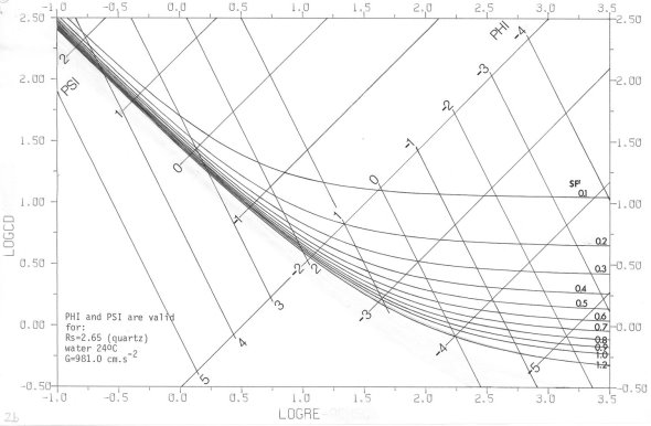
FIG 2: Drag coefficient (logCD) as function of Reynolds’ number (logRe) for various Hydraulic Shape Factor (SF’) values in Nikuradze diagram according to eq. (1); the additional variables PHI-particle size and PSI-settling rate are plotted too as diagonal coordinates. Valid for naturally worn quartz particles sedimenting in distilled water 24°C, gravity acceleration G = 981 cm/sec2 .
(see page 9 for PHI and PSI notations). FIG. 3 reveals a three-dimensional view of the eq. 1; a vertical view (map) in contour (iso)lines is shown in FIG. 4.
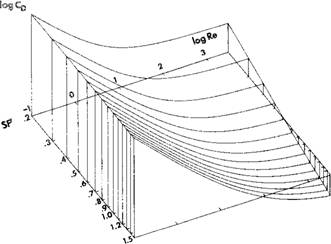
FIG. 3: Drag coefficient (logCD) as function of Reynolds’ number (logRe) and Hydraulic Shape Factor (logSF’); naturally worn sedimenting particles; calculated from the equation (1).
Comparison of some eq. (1) CD values with those by various authors is given in TABLE 2.
|
|
(1) |
(2) |
(3) |
(4) |
(5) |
(6) |
(7) |
(8) |
|
logRe |
log CD |
log CDKASKAS |
Difference |
log CD |
log CDCOLBY |
logCD |
Difference |
|
|
(4) - (5) |
(4) - (6) |
|||||||
|
-3 |
4.3819 3.3869 |
4.3825 |
-,0006 |
4.4762 3.4806 |
|
|
|
|
|
-1 |
2.4029 1.4533 |
2.4032 |
-.0003 +.0000 |
2.4966 1.5634 |
2.415 |
2.537 |
+.082 |
-.040 |
|
1 |
0.6084 0.0108 |
0.6091 |
-.0007 |
0.8409 0.5254 |
0.860 |
|
-.019 |
|
|
3 |
- 0.2741 |
-.2592 |
-.0149 |
0.4473 0.4289 |
0.441 |
|
+.006 |
|
TABLE 2
Data refer to:
column (1): eq. (1), SF’=1.2 (smooth spheres) of this paper;
column (2): KASKAS (1964);
column (4): eq. (1), SF’=0.3 (flat particles) of this paper;
column (5): COLBY + CHRISTENSEN (1956) SF’=0.3 (flat particles);
column (6): KOMAR + REIMERS (1978) SF’=0.3 (flat particles).
SF
log Re
FIG. 4: Contours of drag coefficient (log CD) in terms of Reynolds' number (logRe) and Hydraulic Shape Factor (SF’). Calculated from the eq. 1 using parameters of BREZINA (1977) Naturally worn sedimenting particles.
The drag coefficient values for SF’=1.2 approach very closely those for smooth spheres defined by KASKAS (1964), and even closer experimental data in the range 3<logRe<4. A satisfactory agreement for SF’= 0.3 with the data of COLBY and CHRISTENSEN (1957) and with the equation (14) of KOMAR and REIMERS (1978) is evident (Table 2).
While the Corey's Shape Factor is defined by three particle dimensions only, and the experimental data resulted from studies on naturally worn particles,the smooth spheres have a smaller drag coefficient value than naturally worn irregular particles with SF=1.0 (isometrical particles). This smaller drag coefficient value corresponds to SF’ = 1.2 from the eq. (1). Logically, there is a strong difference between an actually measured SF and the Hydraulic Shape Factor SF’ defined by the regression equation (see page 3).
LOGARITHMIC NOTATIONS OF PARTICLE SIZE (PHI) and SETTLING RATE (PSI).
Retaining the geometric grade scale of J. A. UDDEN (1898), W. C. KRUMBEIN (1934) introduced binary logarithm of particle size, PHI (transcription of the Greek letter φ), which became popular among geologists because it makes calculations and expressions easy. G. V. MIDDLETON (1967) applied the binary logarithm to settling rate, and defined PSI (transcription of the Greek letter ψ):
PHI = -log2Xi , (2a)
inversely Xi = 2-PHI ; (2b)
PSI = -log2Yi , (3a)
inversely Yi = 2-PSI . (3b)
log2 is a logarithm to the base 2 (=binary logarithm);
Xi is a dimensionless ratio of a given particle size, di, in millimeters, to the standard particle size of 1 millimeter, d0 (=di/d0; D. A. McMANUS, 1963; W. C. KRUMBEIN, 1964);
Yi is a dimensionless ratio of a given settling rate, vi, in centimeters per second, to the standard settling rate of 1 centimeter per second, v0 (=vi/v0).
PARTICLE SIZE AND SETTLING RATE EQUATIONS. When rewriting the equation (1), an equation for settling rate v (in centimeters per second) can be written:
K v-2 + L v-1 + M v-0.5 + C = 0 , (4)
if v = X-2 ,
then: K X4 + L X2 + M X + C = 0 .
K = -2-PHI(Rs-Rf) G/Rf . 7.5 ,
L = 10 A . n . 2PHI ,
M = B . (10n)0.5 . 20.5PHI ,
in which:
Rs is the specific gravity of the solid (Rs of quartz is 2.65),
Rf is the specific gravity of the fluid;
Rf of the distilled water varies with temperature; within the temperature range
15°C through 30°C, the following equation has been found satisfactory:
Rfw = a . tb , (5)
in which
Rfw is specific gravity of distilled water under temperature t in ° C (centigrades),
a = 1.013176326
b = -0.0049852
n is kinematic viscosity of the fluid in stokes.
The following equation for the kinematic viscosity of distilled water, developed by Dr. R. E. Manning of the Cannon Instrument Company (MARVIN, 1979) may be used:
nw = nw20.exp {[B0 (t-20) + B1 (t-20)2] /[B2 + t]} (6)
in which
nw20 is kinematic viscosity of distilled water under 20°C; it is taken
0.010038 stokes; the pertinent literature is evaluated by NAGASHIMA (1977);
B0 = -2.930861
B1 = -0.00179426
B2 = 100.495
exp z is exponential function ez, in which e is the basis of natural logarithms, 2.71828…
G is acceleration due to gravity; the standard gravity agreed at the 1968 CGPM (Nature [GB] 220, p. 651, 1968), is the value at Potsdam, 981.260 gal .
The settling rate v can be calculated as a real positive root of the equation (4) by a numerical method; the computer of the Macrogranometer employs the halving method which converges fastest.
The equation (1) can be rewritten into an equation for particle size d (in millimeters):
P d-2 + R d-1 + S d-0.5 + C = 0 (7a)
if d = Y-2 ,
then: P Y4 + R Y2 + S Y + C = 0 .
in which
P = -(Rs-Rf).G.22PSI/7.5 Rf
R = 10.A.n.2PSI
S = B.(10n)0.5.20.5PSI
The equation (7a) can be formulated for PHI-particle size:
P . 2-PHI + R . 2PHI + S . 20.5PHI + C = 0 . (7b)
HYDRAULIC SHAPE FACTOR (SF’) CALCULATI0N. From a known particle size and settling rate, the Reynolds’ number and drag coefficient are calculated:
Re = vd/10n = (2-PHI-PSI) . 10n (8a)
CD = d . (Rs-Rf) G/7.5 Rf .v2 = (22PSI-PHI).(Rs-Rf) G/7.5 Rf (8b)
The Re and CD values are entered into the eq. (1), which can then easily be solved for SF’. This method has been used for construction of the diagrams in FIG. 7, and in the SHAPE program section of the Macrogranometer.
particle size
FIG. 5: Influence of particle shape (SF’) onto the PSI-settling rate plotted as function of the PHI-nominal diameter; naturally worn irregular particles sedimenting in distilled water 24°C, under gravity acceleration G = 981 cm/sec2; calculated from the eq. (4); four diagrams for four density values of particles:
a) Rs = 2.5 b) Rs = 5 c) Rs = 10 d) Rs = 20
FIG. 6: Influence of specific gravity of particles (Rs = 2.5; 5; 10; 20) onto their PSI-settling rate plotted as function of their PHI-nominal diameter; naturally worn irregular particles sedimenting in distilled water 24°C, under gravity acceleration G=981 cm/sec2; calculated from the eq. (4); four diagrams for four SF’ shape values of particles:
a) SF’= 0.15 b) SF’= 0.3 c) SF’ = 0.6 d) SF’ = 1.2
FIG 7: Hydraulic Shape Factor (logSF’) as function of PHI-particle size and PSI-settling rate; naturally worn irregular particles sedimentinq in distilled water 24°C under gravity acceleration G = 981 cm/sec2; data calculated from the eq. (1):
a) Rs = 2.5 b) Rs = 5 c) Rs = 10 d) Rs =20
INFLUENCE OF OTHER FACTORS THAN PARTICLE SHAPE ON THE SEDIMENTATIONAL PARTICLE SIZE ANALYSIS
While the particle shape strongly affects the particle size calculated from settling rate, influence of other variables is less important.
STATIC FACTORS.
Particle size is calculated by 0.01 PHI coarser, if the following terms are effective:
Water kinematic viscosity, n, is lower by -0.0001 stokes
(maximum effect with fine and spherical particles);
caused by: a) temperature is higher by about +0.5°C in average
b) water impurities, particularly by microorganisms (such as algae) salt, etc.
Water specific gravity, Rf, is lower by about -0.003 (maximum effect with coarse and non-spherical particles);
caused by: a) temperature is higher by about +12°C in average,
b) water impurities, particularly due to salt and clay.
Gravity acceleration, G, is higher by about 1 gal (maximum effect with non-spherical coarse particles).
Conclusions: a) A strong observance of water cleanliness is recommended;
b) Water temperature should be watched with ±0.25°C accuracy;
c) Gravity acceleration should be known within ±0.25 gal accuracy.
DYNAMIC FACTORS causing water streaming introduce serious errors if a slow sedimentation (fine, light-weight or non-spherical particles) is involved.
Two main reasons of streaming are recognized:
a) Temperature influence, such as heating, eg by radiation onto a lower, or cooling, eg by evaporation in the upper part of the settling tube. Instable stratification with a negative temperature gradient as low as -0.01°C/cm in a wide settling tube can cause streaming with a velocity which approaches the settling rate of eg. 0.05mm quartz particles (about 0.2 cm/sec). Because the static water temperature influence is much less important, a positive temperature gradient within the settling tube is recommended: +0.005 to 0.05°C/cm.
b) Sedimenting suspension influence from excessive sample size sedimentation. A minimum sample size defined by statistical representativity (BREZINA, 1970) is inevitable. Analyzing large samples in parts (splits) is suitable particularly for coarse material. The Macrogranometer program segments "Split Cumulation” and "Mean" make this technique fast and easy.
- Details
- Last Updated on Saturday, 29 June 2013 07:54
Products & Services |
PRODUCTS
We are offering two sand sedimentation product types:
- Two unique lab instruments:
- Sand Sedimentation Analyzer™, SSA™, MacroGranometer™;
- Sand Sedimentation Separator™, 3S™;
- Various software.
- Details
- Last Updated on Friday, 23 August 2013 21:04
Products & Services | Products
PRICES
We have kept our EURO prices stable since the introduction of the EURO currency (€, EUR) in 2002. For a price estimate in your currency (at the current exchange rate), click the small down arrow on the right side of the "Select Your Currency" toolbar in the Price Table below.
The total cost of our Sand Sedimentation Analyzer (MacroGranometer™ 2013), is 54,555 €, and that of our Sand Sedimentation Separator™ 2013 (3S™), is 61,200 €. These figures include five on-site days for our installation work and personnel training, but not our travel expenses, food and lodging. Also not included is the cost of the Base and Elevated Operation Platform, shipping costs, and customs duty. Most clients themselves can more economically produce the Base and the Elevated Operation Platform. However, for an additional 5,110 € , we can include our installation of a Base and Elevated Operation Platform, all travel, and transportation costs in Europe. If you purchase both instruments at the same time, a 5% discount on both instruments is available.
The SedVar™ data processing software is included in the MacroGranometer™ system.
SedVar™ is also available separately for 2,455 €. Our Shape™ software is 2,550 €.
Price Table
Currently, we could not integrate a currency converter into this page, www.granometry.com .
However, we have it on our old http://www.grano.de/products.htm#prices . Oanda currency converter is here (click).
| # | The Rate of Czech Koruna for 23-AUG-2013 is: Short Description 25.641 CZK/€UR |
€UR |
Select Your Currency |
| 1 | Standard Sedimentation Analysis of your data (minimum of 10 analyses) 10 each. | 10 | |
| 2 | Standard Sedimentation Analysis of your samples (minimum of 10 samples) each. | 49 | |
| 3 | SedVar ™ Number Conversion & Table Generation software; useful for anybody. | 360 | |
| 4 | SedVar ™ Distribution Processing software of the ASCII files generated by the MacroGranometer™ (item 3 is included). | 2455 | |
| 5 | Shape ™ Program; processes both the MacroGranometer ™ and sieving data (ASCII files). By their matching, it can calculate the variable SF (Shape Factor) values. | 2550 | |
| 6 |
Base & Platform for item 7 (MacroGranometer™) or for item 8 (3S ™) — includes installation, travel and transportation in Europe. Most users can more economically produce and install this option themselves following our CAD drawings and instructions. |
5110 | |
| 7 | Sand Sedimentation Analyzer 2013 (SSA, MacroGranometer 2013™), complete analyzing system — includes the instrument's Measuring, Operation and Distribution Processing Software (SedVar™, items 3 and 4) — but not the items 5 and 6. | 54555 | |
| 8 | Sand Sedimentation Separator 2013 (3S™), complete separation system — includes installation, travel, and transportation in Europe — but not the item 6. | 61200 |
MasterCard & VISA accepted.
- Details
- Last Updated on Saturday, 29 June 2013 07:53
Products & Services
USERS
We have been constantly developing our products as the technology permitted. This has resulted in various stages of our instruments evolution.
We have three types of users:
- Users of our products,
- Users of our services,
- Users who identify themselves with our products so much, that they think our products or methods are "theirs". We only wish that they do not forget us — the source they copy, and — that they quote this source at least. Those users of our products or methods, who do not quote us — the source — are "plagiarists".
- Details
- Last Updated on Saturday, 29 June 2013 07:52
Products & Services | Products | ISO Standard
ISO Terms for Sand Sedimentation Balances
Currently, the ISO working group (WG2) of technical committee TC24 has prepared a working draft — "Determination of particle size distribution by gravitational liquid sedimentation methods - Part 4: Balance method". The convener of WG2 has invited me to participate as an expert in this field.
My special task is to define standards in the range of the transitional sedimentation regime, i.e., in the region between the Stokes' law and Newton's law. For quartz density particles sedimenting in water and similar liquids, the range is valid for sand-sized particles, and the sedimentation must be stratified (from one level into clean liquid, line-start methods).
The sedimentation of a single particle is the most accurate method for determining the size of a particle if we are aware of all influencing factors:
- Size definition must be independent of non-spherical (irregular) particle shape.
The volume-equivalent sphere diameter dn of an irregular particle, the nominal volume diameter (Hakon WADELL, 1934), is independent of particle shape. It equals:
dn = (6.V/π)1/3 where V is particle volume. - Sedimentation methods employ the equivalent of a sphere settling in the same liquid and under the same acceleration due to gravity using formulas for settling velocity valid in the given flow regime, such as:
a) by George Gabriel STOKES (1845): spheres sedimenting in laminar flow (small Reynolds’ number, usually 10-7<Re <0.1);
b) by A. A. KASKAS (1964): spheres sedimenting in laminar, transitional and impact (Newton) flows (10-7<Re <104);
c) by Jiri BREZINA (1977, 1979): shape factor (SF) defined irregular particles (sedimentation equivalent to a rotational ellipsoid) sedimenting in all regimes (10-7<Re<104).
However, in the sedimentation of more particles, the particles will mutually affect the sedimentation of each other. These additional particles in suspension will increase both the suspension density and viscosity, in proportion to their instantaneous local concentration and particle surface area.
Generally, a sample of particulate solid material should undergo the type of sedimentation, in which the following factors are exactly known:
- The nature of the acceleration, which moves the particles, such as gravitational or centrifugal acceleration.
- The instantaneous local particle concentration.
- The particle surface area – which is important when dealing with fine and/or markedly non-spherical particles.
In sedimentation balances, acceleration is due to gravity and therefore easy to determine. The instantaneous local particle concentration is the main problem.
Sedimentation balances designed for fine particles such as those by SARTORIUS, GALLENKAMP, METTLER, CAHN and other companies, operate within the laminar (Stokes’) regime (10-7<Re <0.1 or 0.3). In this case, the settling particles do not have sufficient force to overcome the viscous force of the liquid and to separate from each other.
To maximize the mutual distance among the particles, Sven ODÉN (1915) suggested homogenizing the suspension in the sedimentation column. This homogeneous suspension avoids a hydrodynamic instability: every level of the column has the suspension density, which, starting at a zero vertical gradient, becomes increasingly positive as sedimentation proceeds. In other words, the suspension density does not decrease but increases downwards during settling.
However, the sedimentation length of particles is known only for those particles that started at the top. To mathematically subtract the particles with an unknown sedimentation length, the first derivative of the sediment weight accumulating on the balance pan (sedimentation function/curve) must be recorded.
The sedimentation of a homogeneous suspension includes the following disadvantages (error sources):
- The majority of the particles has an unknown sedimentation length.
- The particles with a known sedimentation length are those that started at the top of the column. They are descending most rapidly and therefore they all must pass slower particles, that are hindering them.
- The suspension density and viscosity are increasing downwards with the particle concentration, which is also increasing downwards during sedimentation.
The balance pan collects the sediment and creates a suspension shadow of particle-free (clear) liquid below the pan. The lower density of this liquid introduces a hydrodynamic instability. With the growing concentration of particles suspended above the pan, the clean liquid induces a buoyant force pushing the pan upwards and increases with the progress of sedimentation. The shadow below a balance pan in a homogeneous suspension decreases the sediment load.
Kurt LESCHONSKI (1962, Staub, vol. 22, p. 475) has developed a device, which compensates the buoyancy (German patent). Use of his compensation method is inevitable even for balance pans that have a protective cylinder at the pan's edge (such as that shown schematically in Figures 1 and 2 of the Proposal).
Of course, the clear liquid that is overlain by the homogeneous suspension above the pan will flow upwards (as bubbles) around the pan. This will then cause streaming errors within the overlying suspension. However, using the Leschonski's compensation tube - an equal volume of the overlaying heavier suspension can flow down to replace the volume of the clear liquid.
Sedimentation balances for sand-sized particles, such as the Sand Sedimentation Analyzer™ (MacroGranometer™) by Granometry (Jiri BREZINA, 1969 through 1979), may attain the highest precision level: they operate within the transitional hydrodynamic regime (0.1<Re<3.104), in which the particles have enough force to overcome the viscous force of the liquid, separate from each other and ultimately settle with less dependency on each other. This is the reason why the sand-sized particles are not required to sediment in a homogeneous suspension: the sample can be introduced for sedimentation at the uppermost level of a clear liquid (line-start method - term introduced by Brian H. KAYES, 1969). Then the concentration of particles will rapidly decrease as they settle. Suspension streaming can then be restricted up to the uppermost 5 cm of the sedimentation column. This type of suspension and sedimentation is referred to as stratified because each layer contains particles that have the same sedimentation velocity.
Synonyms:
Settling Tube - used in America, Europe, most countries of Asia
Sedimentation Tower - used in Australia and New Zealand, rarely in GB.
A sedimentation balance for sand-sized particles consists of the following parts:
http://www.grano.de/analyzer.htm
Stratified sedimentation/suspension is described:
http://www.grano.de/article1.htm#stratsusp
Advantage of Stratified Over Homogeneous Sedimentation
Particles settling in groups must be allowed to sediment at mutual distances such that their settling velocities become close to those of single particles. Sedimentation of coarse (sand-sized) grains in water generates forces which liberate the grains from each other: these forces surpass viscosity of the water because the Reynolds' number of the particle is greater than 0.1. Therefore, the coarse grains need not be homogenized for sedimentation, but can be introduced at the top of a particle-free clear fluid. Particles become distributed vertically according to their settling velocity, which is identical for particles at each level: as a result, the so called stratified suspension develops (H. J. Skidmore, 1948, ref. 98; John S. McNown and Pin-Nam Lin, 1952, ref. 90), and stratified sedimentation takes place.
Stratified sedimentation enjoys fundamental accuracy advantages over homogeneous sedimentation. First, the sedimentation length of all particles is known in a stratified suspension. In homogeneous suspension, the sedimentation length is known only for the topmost particles at the beginning of sedimentation; other particles interfere with them and their weight must be eliminated mathematically by taking a derivative. Secondly, the particle concentration (and thus the amount of particle interference) rapidly decreases in the expanding volume of stratified suspension, but it increases toward the bottom of the homogeneous suspension.
A sedimentation balance for sand-sized (0.05 – 4 mm quartz density) particles that uses stratified sedimentation consists of the following parts (see figures here: http://www.grano.de/analyzer.htm ):
- A settling tube composed of glass modules (ISO 3587/1976, 4704/1977), flanges and gaskets as defined in EN 12 585), vertical tube with an inner diameter of 20 cm; a horizontal tube (inner diameter of 30 cm) of a cross piece needed to accommodate an underwater electronic balance. The settling tube provides a sedimentation distance of 180 cm (measured from the Venetian blind lamellae to the top of the balance pan). The glass walls provide both the needed vibratory and thermal stability.
- A Venetian blind for release of the sample and dispersion of particles in the upper 5 cm of the settling tube. After the lamellae open, they vibrate at about ±5° around their vertical position, and at a frequency of 10-20 Hz. 25 lamellae (each 20 cm long, 0.7 cm wide, 0.03 cm thick) are covered by 0.7 cm of water. After the sample is dispersed onto the closed lamellae, the water surface must be covered by a rigid plate allowing no air bubbles to form: this avoids vibrations, which could be formed by waves on a free, uncovered water surface. In addition, the closed water surface prevents evaporation of the water which cin turn could cool the top of the water and thereby cause streaming.
- An underwater electronic balance, with a balance pan of 26 cm in diameter. The balance sensitivity: ±0.01 % of the sample mass of 0.1 – 5 gram. The balance response should be fast (at 30 millisecond for 99 % of the total weight) to record the fastest particles (at 30 cm/sec). Therefore, the underwater weight of the sample must depress the pan by a minimum (maximum 0.1 millimeters by the 10 gram of a mass of quartz). If a spring balance is used, the spring must be very rigid. This permits unhindered sedimentation in the 20 cm wide sedimentation column (this is the width that requires the 26 cm maximum diameter pan).
- Shock absorbers for holding the settling tube and insulating it from environmental vibrations (frequencies >20 Hz should be eliminated).
- The Balance electronics must provide a high quality digital signal with the highest possible signal-to-noise ratio (S/N greater than 90 decibel).
Room temperature
The temperature of the immediate surroundings should not change during the course of the analysis (maximum 20 minutes). Neither should the air temperature vary by more than ±0.5 °C (Celsius temperature is more suitable than Kelvin, because it is identical for differences) during the analysis. To avoid water streaming in the settling tube, a positive vertical temperature gradient of at least +1° C/meter is required. A local vertical gradient of as much as 1° C/cm in the upper 5 cm of the sedimentation column will counteract streaming when the sample is introduced.
However, special care must be taken to avoid any infrared radiation onto the settling tube, i.e. IR radiation from any warmer object in the vicinity of the tube, especially onto its lower part.