
- Details
- Last Updated on Saturday, 29 June 2013 07:51
Calibration Experiment
for IUGS-COS Working Group on Modern Methods of Grain Size Analysis, 1986 - 1989,
chaired by James P. M. Syvitski
|
J. Brezina collected and processed the data of the Experiment from 17 participants, however, he did not complete the final processing before the publication deadline of the book by J. P. M. Syvitski (click on the author's review of the Syvitski's book in Basin Research 4/1992). Below are shown the calibration results of one of the MacroGranometer™ users, the participant No. 14 (in the Syvitski's book quoted under instrument code ST3), in comparison with a precision 0.25-PHI sieving, made by participant No. 7. The calibration samples eliminated the influence of irregular particle shape of natural sand by using glass spheres separated by heavy liquids into narrow density fractions in order to exactly know the density of each of the five mixture components. All available glass spheres had variable density caused by variable amount of fluid and silver-particle inclusions. Three sand samples were mixtures of up to three glass sphere components. J. Brezina produced each mixture component on 65-millimeter screens featuring galvanically deposited meshes with circular holes, with the aid of random vibration of the glass spheres in alcohol suspension on each screen. The minimum material on each screen enabled that only one-layer of spheres has been screened until constant amount of retained spheres (zero throuput), which resulted into ample sieving time. The component portions have been obtained on a high precision rotational sample splitter using the slowest possible samples' flow. The high statistical representativity of each split was confirmed by the negligible variation of the weight of each component split. Still, each sample had specific percentages of each of the three components, and, this way, each sample split was unique for each participant. The percentages of each three sieve fractions of the Sand 1 are shown in the Table below, column headed by "14" for the Participant 14 (Syvitski's code "ST3"), who analyzed the sub-sample [split] 4, = "14S1S4") by the MacroGranometer™. This sub-sample had a mean density 2.487125 g/cm3. For comparison, three sieve fraction percentages of the Sand 1 are shown in the same Table, column headed by "7" for the Participant 7, who analyzed the sub-sample 2 by a carefully executed sieving at 0.25 PHI, however, with woven sieves. |
| Participant-# | 14 | 7 | |||
| # | PHI-mean | mm | g/cm3 | % | % |
| 1 | 0.515±0.010 | 0.700±0.005 | 2.5050 | 25.3 | 26.0 |
| 2 | 1.000±0.015 | 0.500±0.005 | 2.5035 | 20.7 | 20.6 |
| 3 | 1.498±0.020 | 0.354±0.005 | 2.4700 | 54.0 | 53.4 |
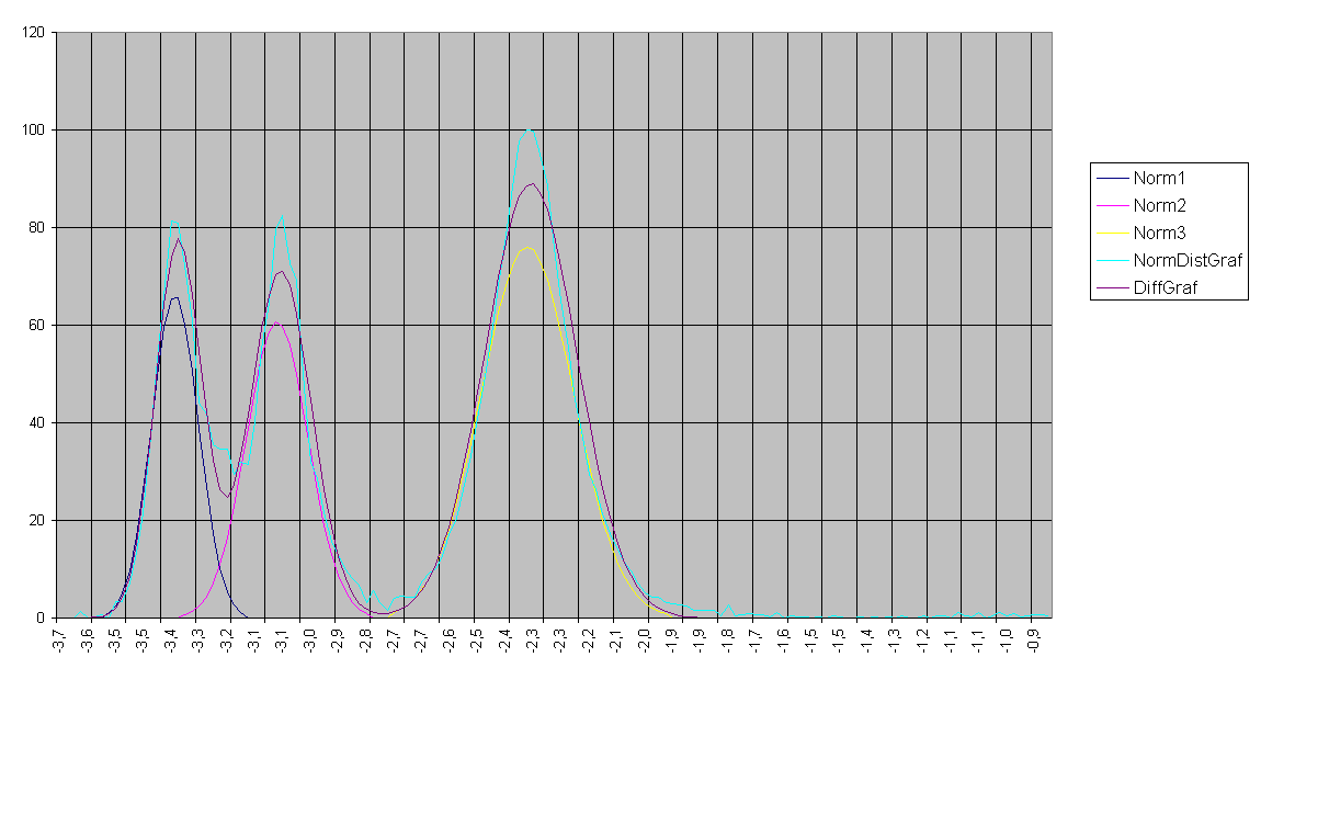
The MacroGranometer™ analysis by the participant 14 of the same sample (Sand 1), and decomposed
by our program Shape™, has recovered the original three distribution components very closely:
| # | PHI-mean | mm-mean |
PHI-standard deviation |
% |
| 1 |
0.5840 |
0.667 | 0.0698 | 22.39 |
| 2 | 0.8733 | 0.546 | 0.0842 | 26.99 |
| 3 | 1.4926 | 0.355 | 0.1053 | 50.63 |
Below: graphical plots of the MacroGranometer™ analysis.
The sample 14S1S4 was a calibration material consisting of glass spheres,
participant 14 ("ST3"), sand 1, sub-sample (split) 4 = 14S1S4.dat .
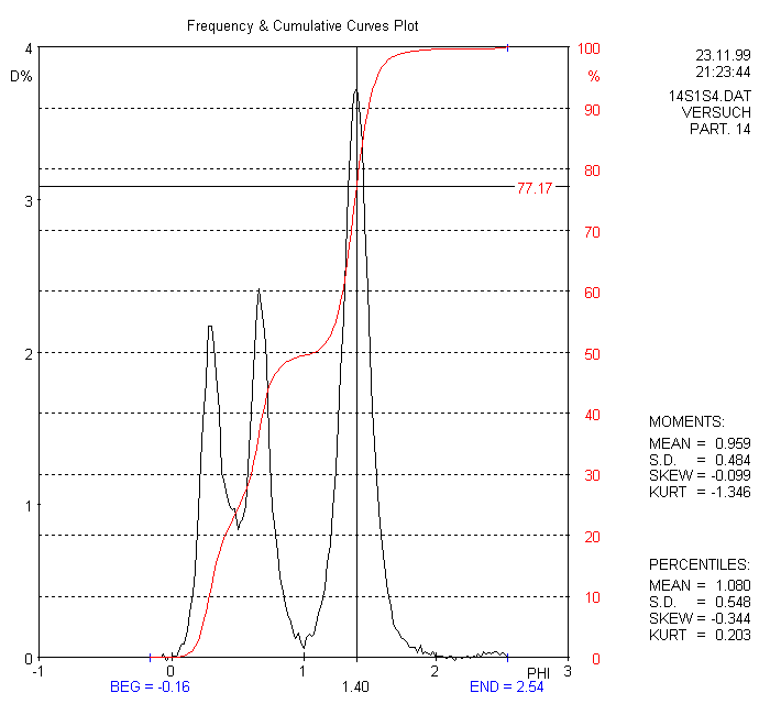
Above: example of an analysis processed by SedVar™ into frequency and cumulative curves
— the frequencies are plot in linear scales.
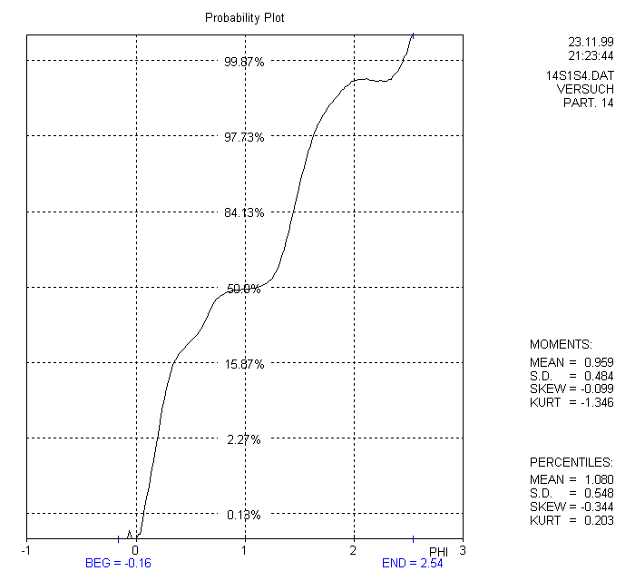
Above: example of an analysis processed by SedVar™ into cumulative curve
— the cumulative frequency is in probability scale.
Below: the above sample decomposed into 3 Gaussian components by our program SHAPE™;
the component parameters are the best test of the Analyzer (plot by MS EXCEL© program):
Below: the standard sieving result (at 0.25 PHI intervals) by the participant 7 compared with the MacroGranometer™ analysis (at 0.02 PHI intervals) by the participant 14:
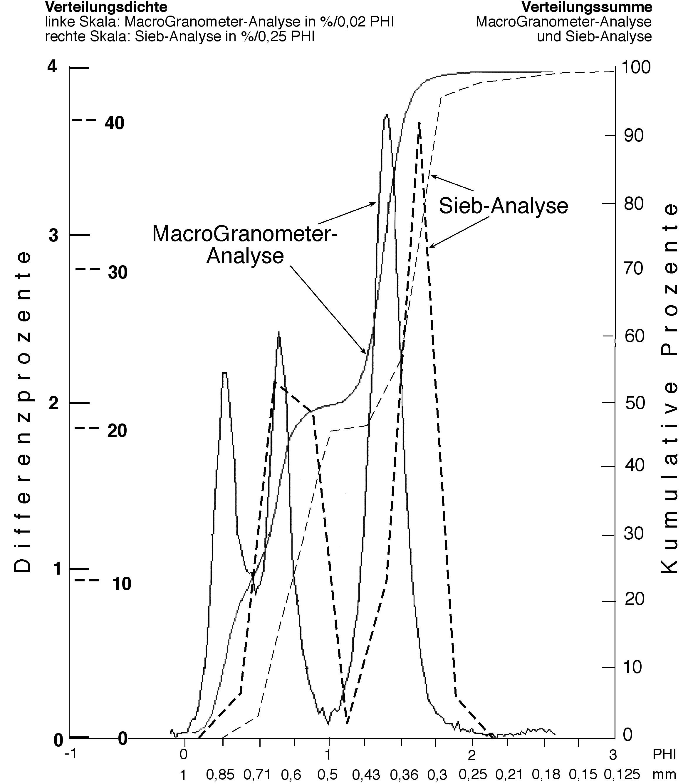
The sieving data (dashed lines) above suffer from three fundamental shortcomings of the sieving (at 0.25 PHI) in comparison with a sedimentation method (at 0.02 PHI):
- The sieving, using 12.5-times wider intervals than the MacroGranometer™, resolves only two instead of three components. The third component can only be suspected according to the asymmetry of the smaller distribution component.
- The sieving is shifting the results by its interval width (0.25 PHI = 1/8 of the grain size) toward finer grain size.
- Nonspherical particle shape affects the sieving size inconsistently with specific surface: nonspherical particles are sieved as coarser, whereas their specific surface is greater as that of the finer particles (this shortcomming was eliminated by using glass spheres).
Please note that Syvitski has not:
-
exactly known the size distributions of the test samples synthesized by J. Brezina, therefore his evaluations were not appropriate;
-
identified the mixed distribution components by a program such as our Shape™.
Calibration Conclusions:
Five types of settling tubes provided clearly better results than all other tested instruments (image analyzer, Coulter-Counter™, Malvern™ laser particle sizer, SediGraph™, photosedimentometer Lumosed™).
From the five settling tubes, three ones (two of them were MacroGranometers™) qualified as Advanced Settling Tubes. The output of both MacroGranometers™ best matched the expected results using the above shown highly demanding criteria (fit of the mixed distribution components).
The other settling tubes, and particularly other instruments, could even not reproduce the original fractions. The component modes were so strongly shifted that they could hardly be recognized as formed by the original fractions; frequently, additional modes formed or some of the modes disappeared.
You are visitor number since July 17, 2000