
- Details
- Last Updated on Thursday, 29 December 2016 02:49
Distribution Decomposition into Gaussian Components
Our program SHAPE™ (based on the method by Isobel CLARK, 1977) decomposes
a measured distribution into the maximum of five Gaussian components
This way, SHAPE™ may define a distribution by (3n-1) parameters (n is the number of Gaussian components):
n means, n standard deviations and n-1 percentages.
We limited the number of components by 5, because we experienced that a higher number of components is not realistic.
Example
A sand fraction of nearly monosized grains, made by precision sieves with circular holes:
SAMPLE FileName: sed122.dat
|
Material: |
beach black sand |
sample 13 |
at a 90° intersection of beaches |
|
Locality: |
near Casusay |
Venezuela Bay |
about 110 km NNW of Maracaibo |
|
Sampling Date: |
1972-5-15 |
low tide |
tide amplitude: about 75 cm |
|
Analysis date, time: |
1981-2-1, 16:55h |
Tmean = 24.76°C |
|
|
Preparation: |
precision wet vibration sieving |
circular holes ± 0,002 mm |
|
|
MonoSized: |
1.770 ±0.0639 PHI |
= 0.297 ±0.013 mm |
|
|
Average of 8 sample |
Total Mass: |
0.6916 gram 0.08645 gram |
SF = 0.63 (calculated Corey‘s Shape Factor) Glab = 980.962 gal (cm/sec2) |
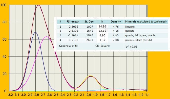
PSI distribution of monosized (1.77PHI=0.297mm) polymineral fraction decomposed into 4 Gaussian components
X (horizontal) axis - PSI
Y (vertical) axis - frequency
Curves: the upper one in dark red is the original mixed distribution,
the four curves below are the resulting Gaussian components as described in the inserted table - from left:
1 dark blue,
2 magenta,
3 yellow,
4 light blue.
Our Sand Sedimentation Analyzer™ (MacroGranometer™), has distinguished 105 (END-BEG) PSI intervals, at 0.02 PSI width (X-axis).
No data manipulation such as “smoothing“ has been used.
The smoothness of the 1st derivative,“Input d%“ (see above), and particularly the extremely small Chi-square χ2 <0.01 show the analysis quality.
In the given example, SHAPE™ decomposed the analyzed PSI distribution into 4 Gaussian components with the following
11 parameters (columns 2, 3 and 4 in the table below, the table is also inserted in the graph above):
4 means, 4 standard deviations, 3 percentages (the 4th one is the rest up to 100%):
|
# |
PSI-mean |
St. Dev. |
% |
Density |
Minerals (calculated & confirmed) |
|
1 |
-2.8095 |
.1007 |
34.56 |
4.76 |
ilmenite |
|
2 |
-2.6376 |
.1645 |
52.15 |
4.16 |
garnets |
|
3 |
-1.9685 |
.1090 |
9.90 |
2.65 |
quartz, feldspars, calcite |
|
4 |
-1.5137 |
.2601 |
3.39 |
2.08 |
porous calcite (fossils) |
|
Goodness of fit |
Chi-Square: |
χ2 <0.01 |
|||
Our program NGRM™ calculated density from the constant PHI size to each PSI-mean value.
The density values of each component match the minerals identified microscopically and by X-ray diffraction analysis.
The Standard Deviation values of the calculated density correspond to many inclusions (in quartz, feldspars, Ca-carbonates) and chemical variations due to isomorphism (ilmenite, garnets).
Our program SedVar™ converted the variable PSI into a log density distribution (not shown here).
Comments
The extremely low Chi-square value, χ2 <0.01, reveals the decomposition quality.
The relatively low values of the standard deviation at ilmenite and quartz, feldspars + calcite corresponds to the relatively monomineral constituents.
The higher standard deviation value at garnets corresponds to relatively wide chemical variability of these minerals.
The high value of standard deviation at porous calcite (fossils) corresponds to great variability of the pores filled by water (the bulk density).
3D Plot
The 3D section of our SedVarDP™ program can arrange the probability curves into a 3D space as shown on this example.
Below, probability curves of 7 narrow fractions are arranged according to their PHI grain size:
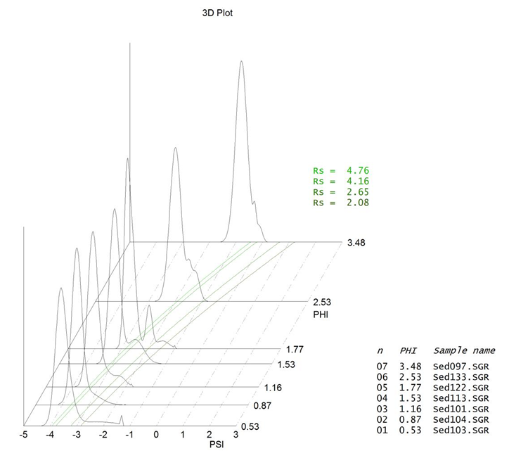
Legend:
X (horizontal) axis - PSI (log settling rate),
Y (perpendicular) axis - PHI (log particle size),
Z (vertical) axis - dF (differential frequency).
Comments
- Seven PSI distribution curves of various PHI particle size and from it calculated density Rs (the variously green curves) are plotted within the X-Y (PSI-PHI) plane.
- The PSI distribution curve at 1.77 PHI displays the best component separation.
The reason is that the PHI-size fraction is the narrowest (pratically monosized).